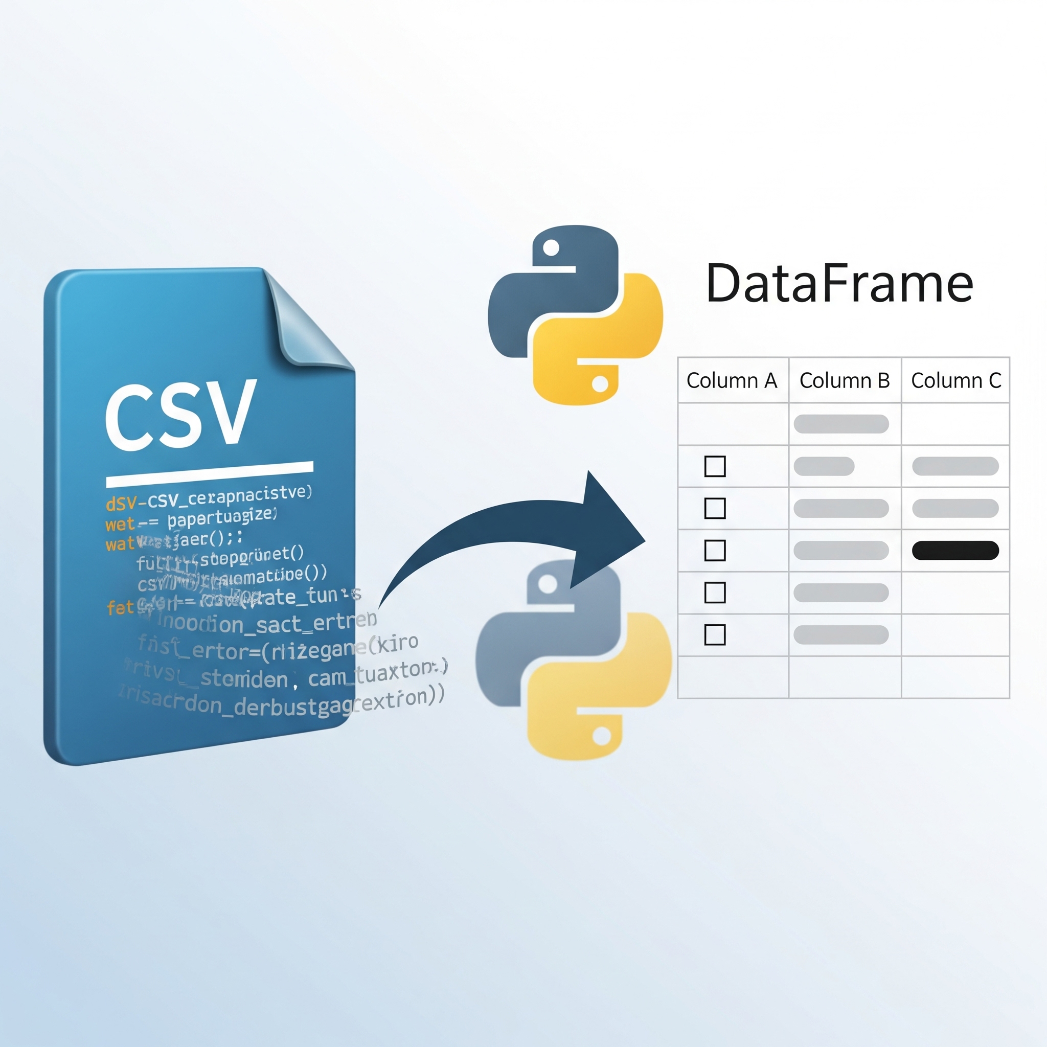
Forecasting future events—from quarterly sales to daily energy demands—is critical across numerous fields. While traditional ARIMA models suffice for straightforward data, real-world datasets often present complexities like seasonality and external factors. SARIMAX offers a robust solution. This model extends ARIMA's capabilities, enabling more accurate forecasts by incorporating seasonal patterns and exogenous variables. ## Understanding SARIMAX SARIMAX, while seemingly complex, is an acronym representing key model components: * **S (Seasonal):** Accounts for recurring patterns (e.g., weekly or monthly fluctuations). * **AR (Autoregressive):** Utilizes past variable values for future prediction. * **I (Integrated):** Handles non-stationary data (data exhibiting trends). * **MA (Moving Average):** Leverages past forecast errors to refine predictions. * **X (Exogenous Regressors):** Includes external factors influencing the target variable. For a deeper dive into SARIMAX, see this [comprehensive guide on datascientest](https://datascientest.com/en/sarimax-model-what-is-it-how-can-it-be-applied-to-time-series). Essentially, SARIMAX enhances ARIMA by integrating seasonality and external influences. ## Forecasting Daily Website Traffic: A Case Study This example demonstrates SARIMAX's application in forecasting daily website traffic, incorporating daily advertising spend as an exogenous variable. Increased advertising is expected to correlate with higher website visits. ## Data Description: `web_traffic.csv` The analysis uses `web_traffic.csv`, structured as follows: <img src={require('./img/Gemini_Generated_dataset_overview.jpg').default} alt="A table visualizing the structure of the web_traffic.csv data, showing 'date', 'visits', and 'ad_spend' columns." width="600" height="350"/> <br/> | Column Name | Description | |-------------|---------------------------------| | `date` | Observation date | | `visits` | Daily website visits (target) | | `ad_spend` | Daily advertising expenditure (exogenous) | ## Building the SARIMAX Model This section details SARIMAX model construction using Python. <img src={require('./img/Gemini_Generated_Image_sarima.jpg').default} alt="A flowchart illustrating the SARIMAX model building process, from data loading and visualization to model fitting and evaluation." width="600" height="350"/> <br/> ### 1. Software Installation Install necessary libraries: Explore further: - Discover practical implementations in this [Kaggle notebook on Time Series Forecasting with ARIMA/SARIMA](https://www.kaggle.com/code/brendanartley/time-series-forecasting-w-arima-sarima). ```bash pip install pandas matplotlib statsmodels ``` ### 2. Data Loading and Visualization First, load and visualize the data to identify trends, seasonality, or anomalies: ```python import pandas as pd import matplotlib.pyplot as plt df = pd.read_csv('web_traffic.csv', parse_dates=['date'], index_col='date') df['visits'].plot(title="Daily Visits Over Time", figsize=(10, 4)) plt.xlabel("Date") plt.ylabel("Number of Visits") plt.grid(True) plt.show() ``` Visual inspection aids in informed model selection. - [statsmodels](https://www.statsmodels.org/dev/generated/statsmodels.tsa.statespace.sarimax.SARIMAX.html) – The official documentation for the SARIMAX implementation in the `statsmodels` library. This resource provides detailed explanations of model parameters, usage examples, and links to the source code. It is essential for understanding the full capabilities of SARIMAX, including advanced options for diagnostics, model selection, and forecasting with exogenous variables. ### 3. Data Splitting: Training and Testing Sets **(Further steps would follow here, detailing model fitting, parameter selection, forecasting, and evaluation.)** ## SARIMAX Time Series Forecasting with Exogenous Variables ## Data Preparation Before model building, the dataset must be split into training and testing sets to evaluate generalization performance. The exogenous variable (`ad_spend`) will also be separated. ```python train = df.loc[:'2024-11-30'] test = df.loc['2024-12-01':] exog_train = train[['ad_spend']] exog_test = test[['ad_spend']] ``` **Important Note:** Ensure the exogenous variables (`exog_train`, `exog_test`) are perfectly aligned with the target variable (`visits`) in terms of dates and contain no missing values. ## 3. Fitting the SARIMAX Model This section details fitting the SARIMAX model and evaluating its performance. This involves selecting appropriate parameters (p, d, q, P, D, Q, s), fitting the model using `statsmodels`, generating predictions on the test set, and evaluating accuracy using metrics like RMSE or MAE. Iterative experimentation and careful consideration of data characteristics are crucial for optimal model performance. For a comprehensive understanding of SARIMAX implementation in Python, refer to the following resource: - [geeksforgeeks](https://www.geeksforgeeks.org/python/complete-guide-to-sarimax-in-python/) – This guide provides step-by-step instructions, code examples, and explanations for building SARIMAX models, including parameter selection and model diagnostics. ## Forecasting with SARIMAX SARIMAX models predict future values by considering trends, seasonal patterns, and external factors. This example uses an ARIMA order of (1,1,1) to capture the underlying trend and a seasonal component (1,1,1,7) to account for weekly seasonality. ### Model Building The SARIMAX model is built using the following Python code: ```python from statsmodels.tsa.statespace.sarimax import SARIMAX model = SARIMAX(train['visits'], exog=exog_train, order=(1, 1, 1), seasonal_order=(1, 1, 1, 7), enforce_stationarity=False, enforce_invertibility=False) result = model.fit(disp=False) print(result.summary()) ``` <img src={require('./img/chat-gpt-inferenced-image-for-the-sarimax.png').default} alt="A line graph showing daily website visits over time, illustrating potential trends and seasonality." width="600" height="350"/> <br/> The parameters are defined as follows: * **(p=1, d=1, q=1):** Autoregressive (AR), differencing (I), and moving average (MA) terms for the trend. These control the model's consideration of past values. * **(P=1, D=1, Q=1, s=7):** Seasonal counterparts capturing weekly patterns. * **`exog=...`:** Includes `ad_spend` (`exog_train`) as an external factor influencing predictions. ### Model Evaluation Predictions are generated for the test dataset: ```python pred = result.predict(start=test.index[0], end=test.index[-1], exog=exog_test) ``` Visualization of model performance would follow here. ## SARIMAX Model Evaluation and Fine-tuning ## Visualizing Model Performance The following code generates a plot comparing actual versus predicted values. The plot visualizes the model's performance during the test period. A close alignment between the green (actual) and red (predicted) lines indicates strong predictive accuracy. ```python import matplotlib.pyplot as plt plt.figure(figsize=(12, 5)) plt.plot(train.index, train['visits'], label='Train Data') plt.plot(test.index, test['visits'], label='Actual Visits', color='green') plt.plot(pred.index, pred, label='Predicted Visits', color='red', linestyle='--') plt.legend() plt.title("SARIMAX Forecast vs Actuals") plt.xlabel("Date") plt.ylabel("Visits") plt.grid(True) plt.show() ``` How well do you anticipate the model performing based on this visualization? ## Quantifying Model Accuracy Standard error metrics provide a quantitative assessment of the model's predictive power. Lower values indicate better performance. Mean Absolute Error (MAE) is particularly useful due to its robustness to outliers. ```python from sklearn.metrics import mean_squared_error, mean_absolute_error rmse = mean_squared_error(test['visits'], pred, squared=False) mae = mean_absolute_error(test['visits'], pred) print(f"Root Mean Squared Error (RMSE): {rmse:.2f}") print(f"Mean Absolute Error (MAE): {mae:.2f}") ``` ## Fine-tuning the SARIMAX Model Experimentation is key to optimizing SARIMAX model performance. While starting with simple (1,1,1) and (1,1,1,7) orders is recommended, adjustments may be necessary. ACF/PACF plots (`plot_acf`, `plot_pacf`) aid in identifying optimal lag values. For automated parameter tuning, consider using `pmdarima.auto_arima()`. Crucially, avoid "future leakage" by ensuring external variables are known *before* the prediction period. ## Applications of SARIMAX SARIMAX is a versatile forecasting tool applicable across diverse fields: * **Marketing:** Forecasting sales based on advertising expenditure. * **Cloud Operations:** Predicting resource demand based on workload and business events. * **Finance:** Modeling stock prices by incorporating macroeconomic indicators. * **Healthcare:** Forecasting patient inflow using seasonality and policy data. In summary, SARIMAX is an ideal forecasting method when modeling trends and seasonality, incorporating external factors, and requiring a statistically sound and interpretable model. In conclusion, this guide demonstrated the power of SARIMAX for building accurate time series forecasts, particularly when dealing with seasonal data and external factors. We explored the components of SARIMAX—Seasonal, Autoregressive, Integrated, Moving Average, and eXogenous regressors—highlighting its advantage over simpler ARIMA models. [nife.io](https://nife.io/) has developed an advanced AI-powered solution to monitor your organization's resource usage, forecast future demand, detect anomalies in real-time, and optimize infrastructure costs — all from a single intelligent dashboard tailored for modern IT operations.